Thanks for your visit, but this page is under translation into English. Sorry...
|
IFTA2013: Spatiotemporal Technical Analysis by T.Suzuki
日本語版は こちらです.
Hello, everyone. I’m Tomoya Suzuki and working at Ibaraki University in Japan. Today, I’d like to introduce my theory, which is Spatiotemporal Technical Analysis. This "spatiotemporal" is my originality for technical analysis.
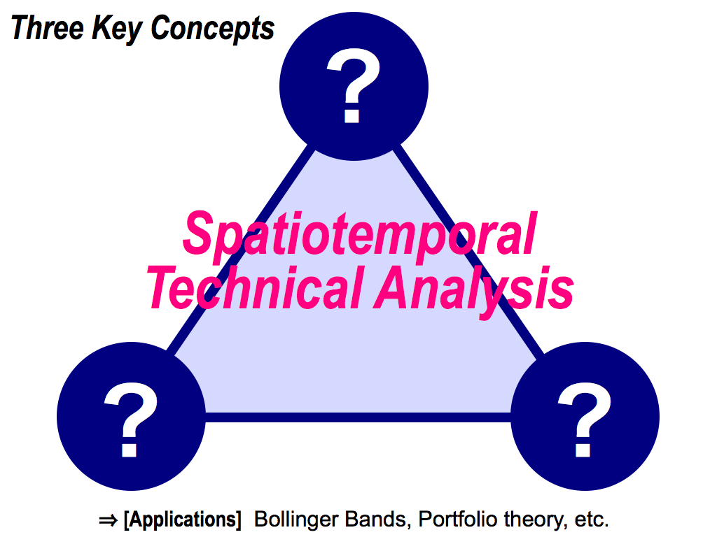
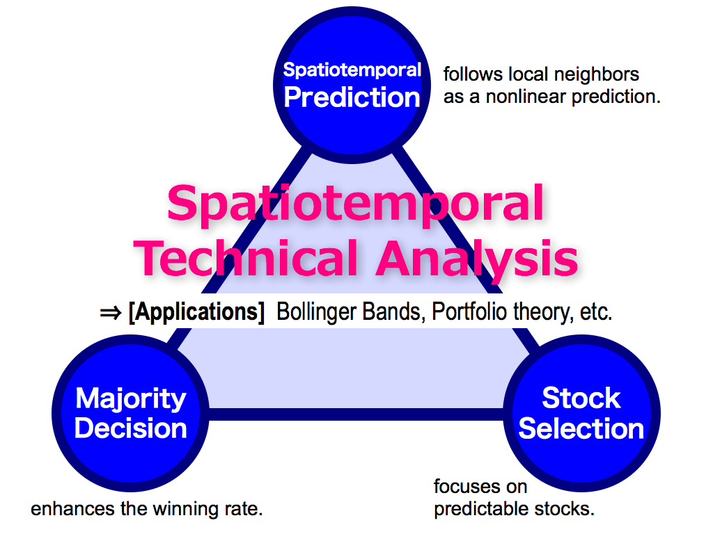
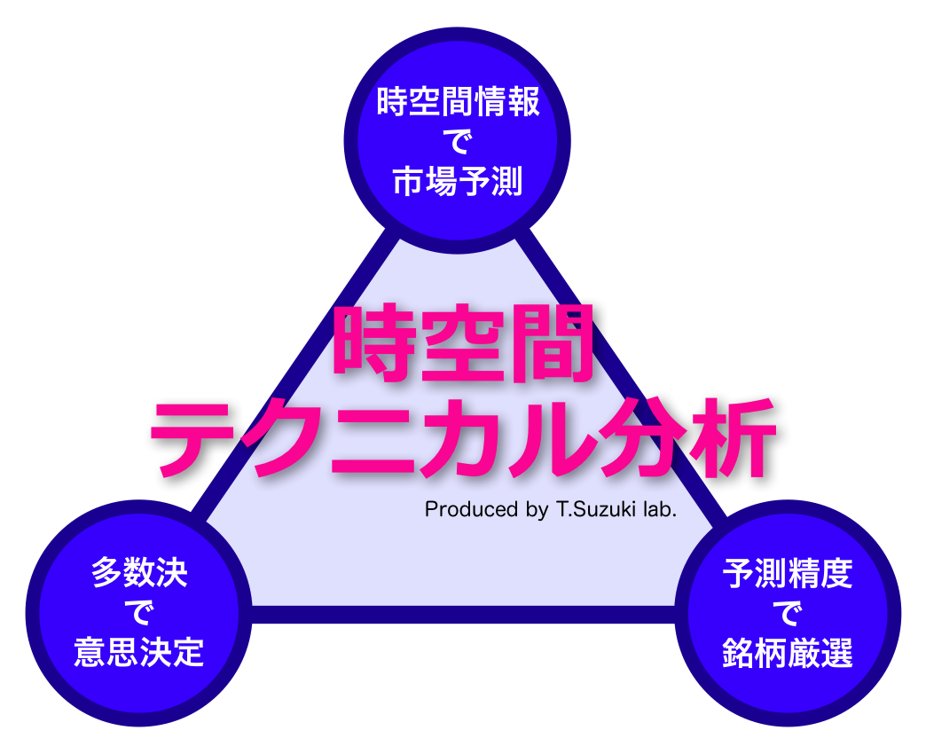
First of all, my theory has three key concepts like this triangle. I will introduce one by one, in the first part of my presentation. And then, I’ll apply my theory to the famous Bollinger bands and the Markovitz’s portfolio theory.
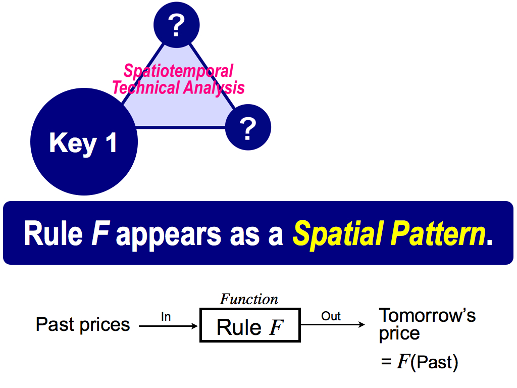
This is the first key. Let’s see a spatial pattern, but I know spatial pattern isn't famous. But, this is based on the chaos theory. Actually, my major is physics, and so I’m familiar with chaos theory.
As shown here, there is a the rule F. This means a mathematical function like this F. The function has some inputs and an output. In financial markets, past prices are inputs to the function F, and you can get tomorrow’s stock price as an output. So, the rule is the relationship between past and future, input and output. If we can know the rule F, we can predict future. But, in general, we don’t know this rule F. So, prediction is difficult.
However, what I want to say is, this first key is very effective to understand this rule F because the rule F appears as a spatial pattern. And then, you can use it for prediction. Why is it? This is the first key.
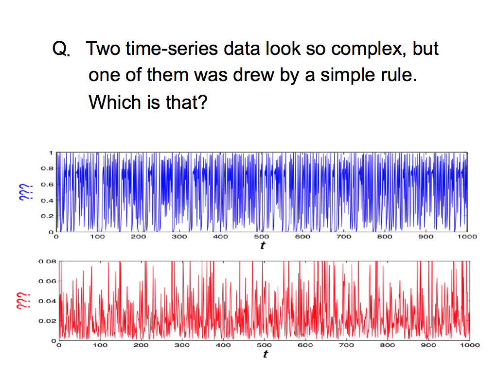
To introduce my idea in more detail, I’d like to ask a question. There are two time-series data, blue and red. Both time-series data look so complex. So, you might think, it’s difficult to understand the rule F deriving these complex fluctuations. But actually, one of them was drew by a very simple rule. I used the simple rule to drow the data. Which is that? Please guess which time-series has a simple rule. To be honest, this question is very difficult for human.
Actually, there is a good convenient technique to solve this question. So, let's change this temporal expression into a spatial expression, like this …
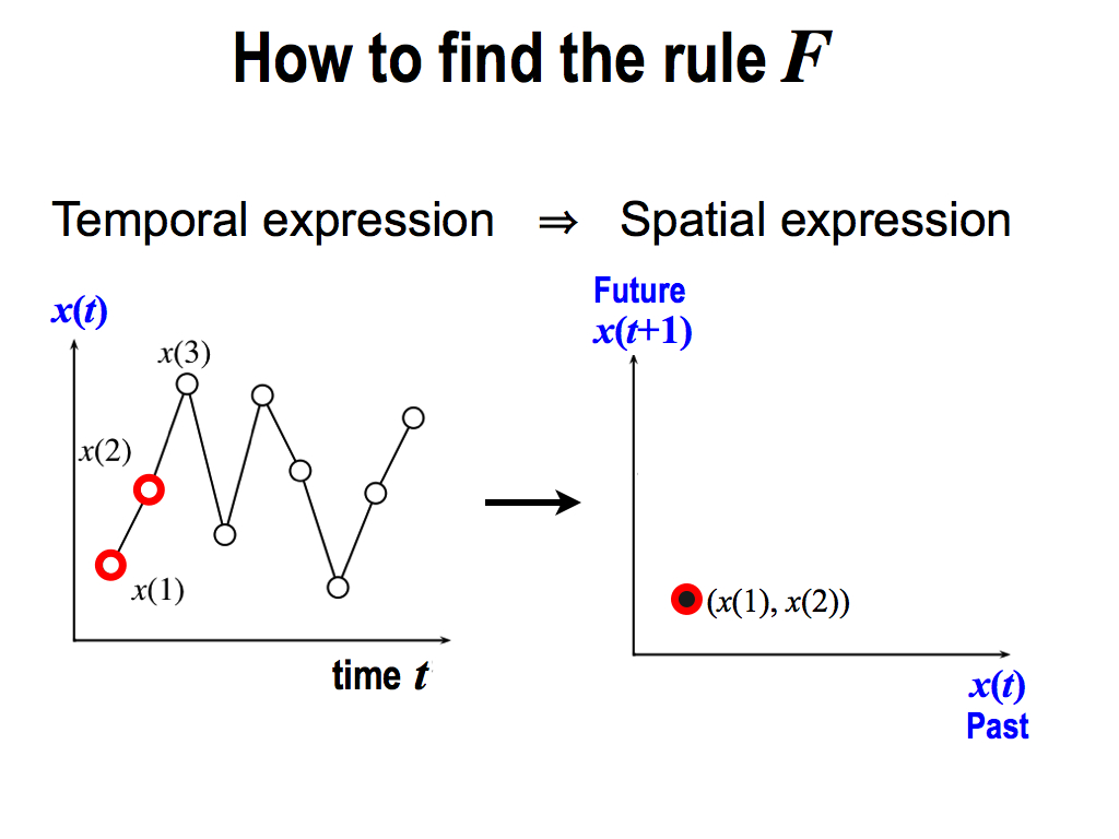
Left figure is the temporal expression, because this horizontal axis is time t. From here, I pick up two data like this. And then, I plot it here. This horizontal value is x(1), and the vertical value is x(2). So, this is just a space composed by only x values, not using time t. That’s why, this is a spatial expression.
On the other hand, this is a temporal expression, because this horizontal axis is time t.
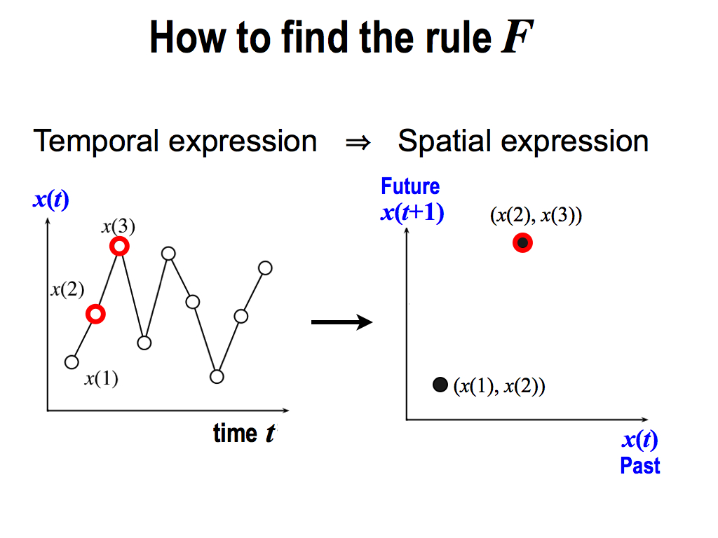
And then, I repeat the same thing, picking up the next two values x(2) and x(3). Then, I plot it in the same space.
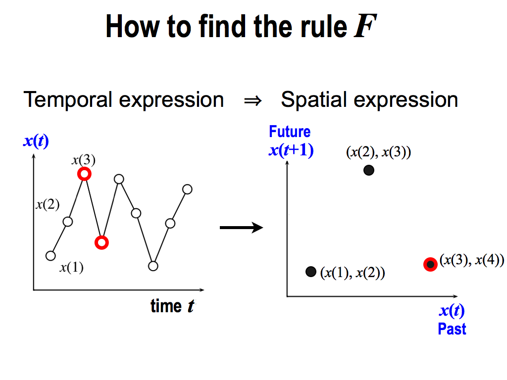
And similarly, I pick up x(3) and x(4), and I plot it again in the same space.
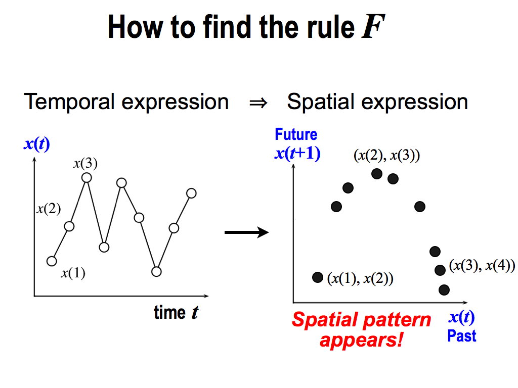
By repeating the same thing, finally, we can see a spatial pattern appears like this. It's amazing!
Here, the most important thing is, this spatial pattern directly corresponds to the rule F deriving this time-series data. So, if you see this spatial pattern, you can understand the detail of the rule F, and you can predict the future. Why is it?
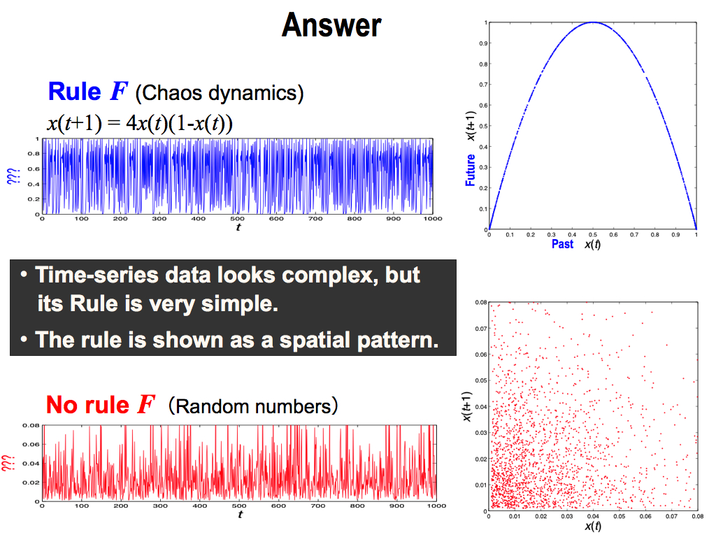
This is the answer. The upper blue data is based on a simple rule F of this function, which is one of famous chaos dynamics, Logistic map. Here, the right side of this function has a past data x(t) as an input, and the left side has a future data x(t+1) as an output. So, this function means the relationship between past and future, inputs and output.
In this sense, this spatial expression means the same thing. This horizontal axis is a past value x(t), and the vertical axis is its future x(t+1). So, this is also the relationship between past and future, inputs and output. That’s way, the rule F was shown here as a spatial pattern.
And, I’d like to show you another evidence. In the right part, there are two x. You can multiply them, and you can get -x squared. As you know, this means a upward convex. It is just this spatial pattern. This is an evidence that spatial pattern can reproduce the rule F by the spatial expression. So, if you use this spatial expression, you can understand the detail of the rule F. And then, you can use it for prediction. That’s why, spatial expression is very important.
On the other hand, the lower red data is based on random numbers. So, we cannot find any spatial pattern, which also concludes this time-series is random.
Here, there are two important conclusions: First, time-series data looks complex, but sometimes its rule is very simple. So, we shouldn’t give up predictions. Second, this rule can be shown as a spatial pattern. Spatial pattern is very important to get the rule F.
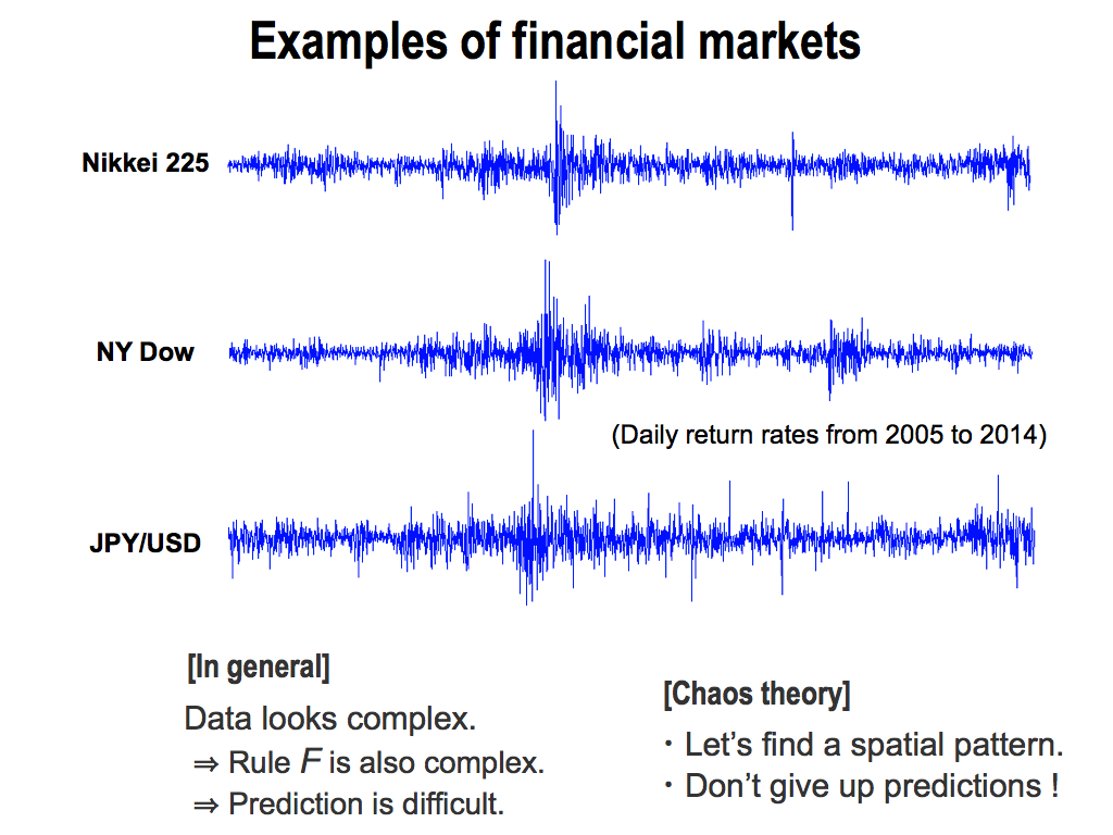
Ok, let me show you examples of real financial markets. These are daily return rates for 10 years of Nikkei index, NY Dow, and Yen-Dollar foreign exchange rates.
As you can see, these data look complex. So, you might think, the rule F deriving these data is complex, and so prediction is difficult. But, please remember chaos theory. Chaos theory encourages us. Let’s find a spatial pattern to understand the rule F. Don’t give up any predictions.
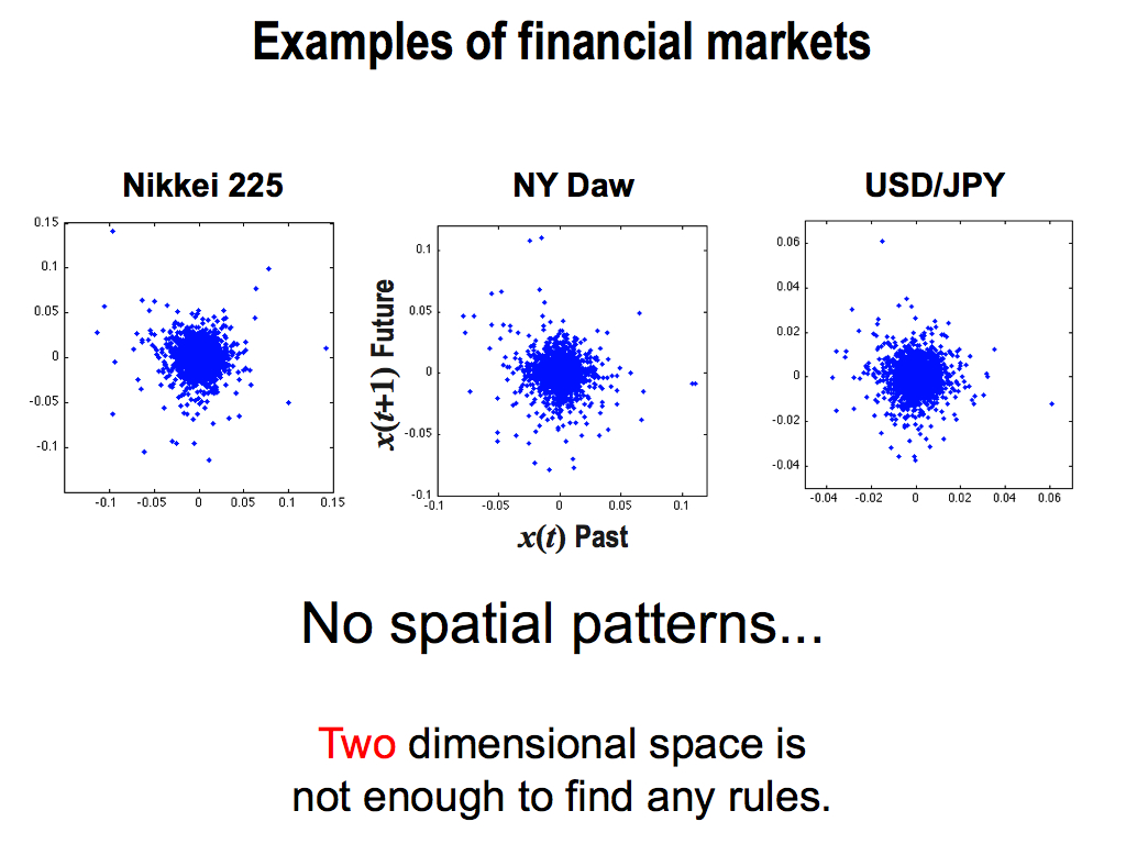
But unfortunately, real markets are difficult to find the rule F because we can see no spatial patterns. Each spatial pattern is overlapped complexly. But I think, these two dimension is too low to find any rules.
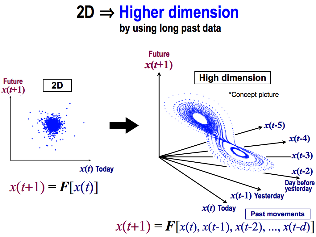
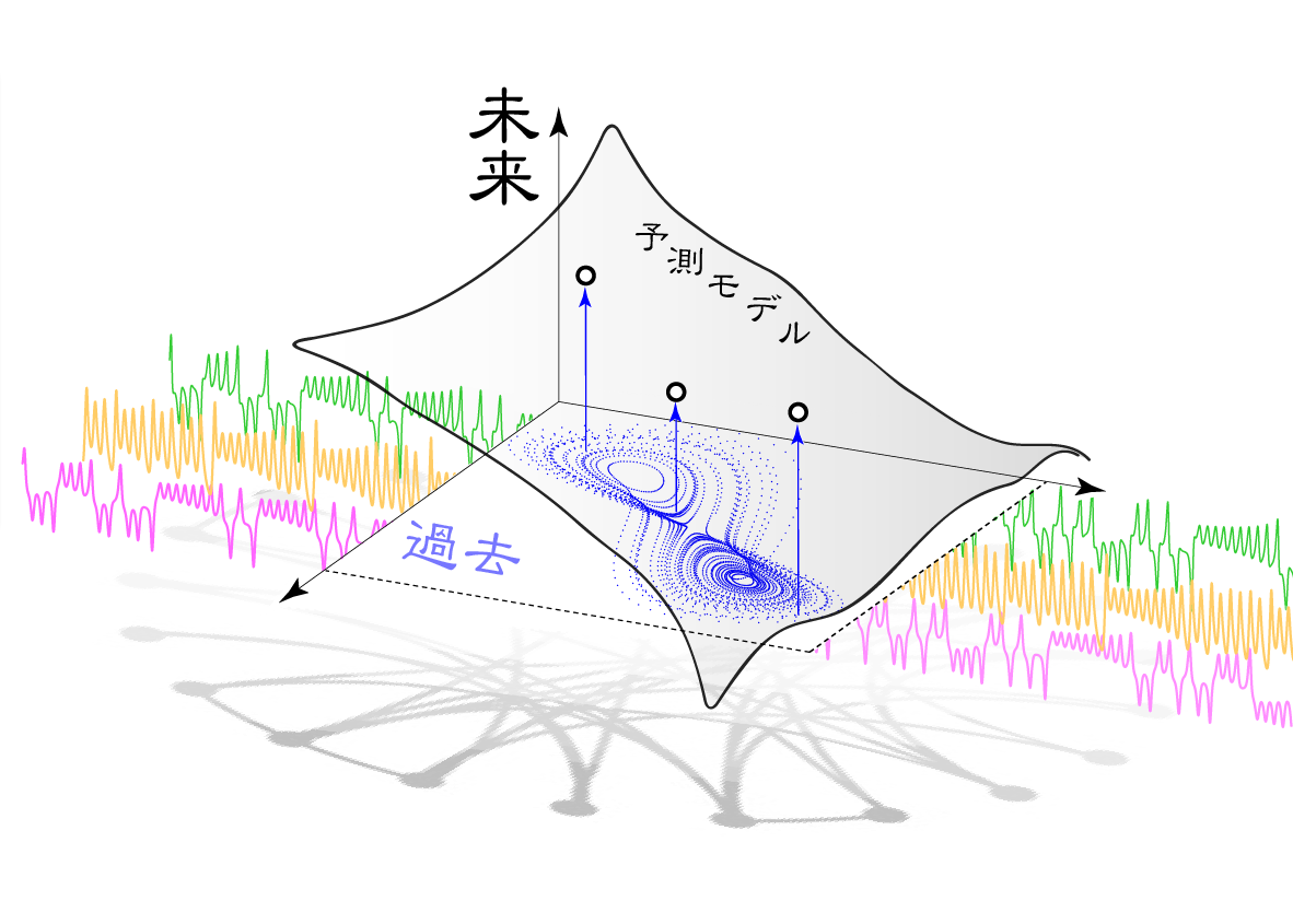
Therefore, we have to enlarge this dimension into two dimension to higher dimension like this. Here, this beautiful spatial pattern is a only concept because we cannot draw more than three dimension. Real spatial pattern might be more complex because real systems are noisy.
To compose this high dimensional space. we have to use long past movements, like these axises. This axis means yesterday’s price, and this axis means the day before yesterday, and so forth.
And, these axises are inputs to the function F, and we can get a future price x(t+1) as an output. So, this spatial expression shows the relationship between past and future, inputs and output. Then, this spatial pattern corresponds to this function, rule F.
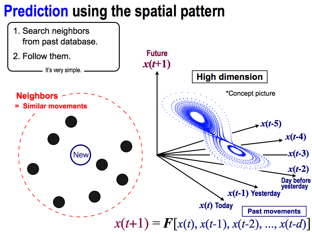
And then, let’s perform prediction by using the spatial pattern. In this case, I want to predict the future of this new point, which is the newest data in this high dimensional space.
Fortunately, this prediction is very simple and easy because what I have to do for prediction is only two things.
First, I search neighbors from past database. These black points are neighbors of the new point. And, these neighbors are similar movements, because each position is decided by these axises, which mean inputs to the function F. So, neighbors are similar inputs to this function F. Therefore, their outputs must be similar. That’s why, each future behavior moves similarly, like this.
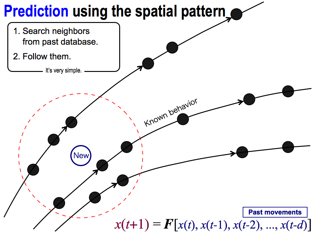
Neighbors go to the same direction. Moreover, we have data of these behaviors because these neighbors were selected from the past database.
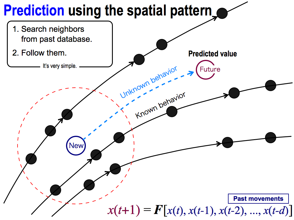
So, I can follow these behaviors to predict the future, like this. This prediction is very simple and easy! And, this prediction is based on the chaos theory.
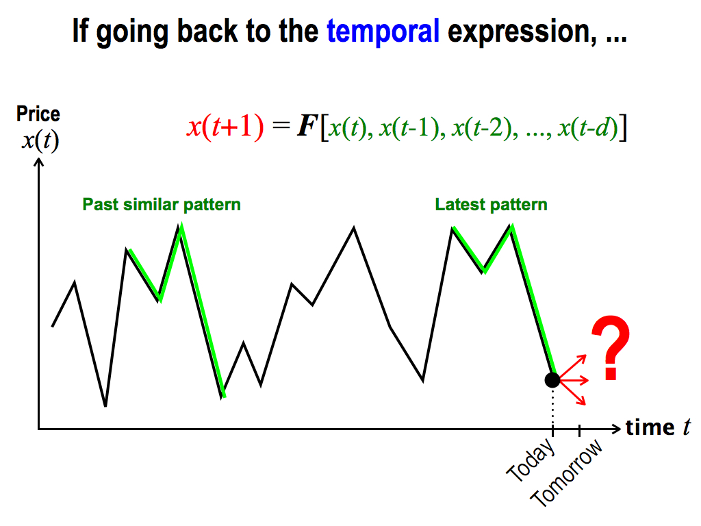
For more familiar expression, let’s go back to the temporal expression, that is, the horizontal axis is time t.
Here, I want to predict the tomorrow’s price. This is today, and tomorrow is unknown. So, I want to predict this.
So, I find out a past similar pattern to the latest pattern. In this case, this dimension d is four, because one, two, three, four. That’s, four dimension, if we use a spatial expression. But, Now is a temporal expression because the horizontal axis is time.
Then, these similar patterns are the similar inputs to this function. Therefore, their outputs move similarly.
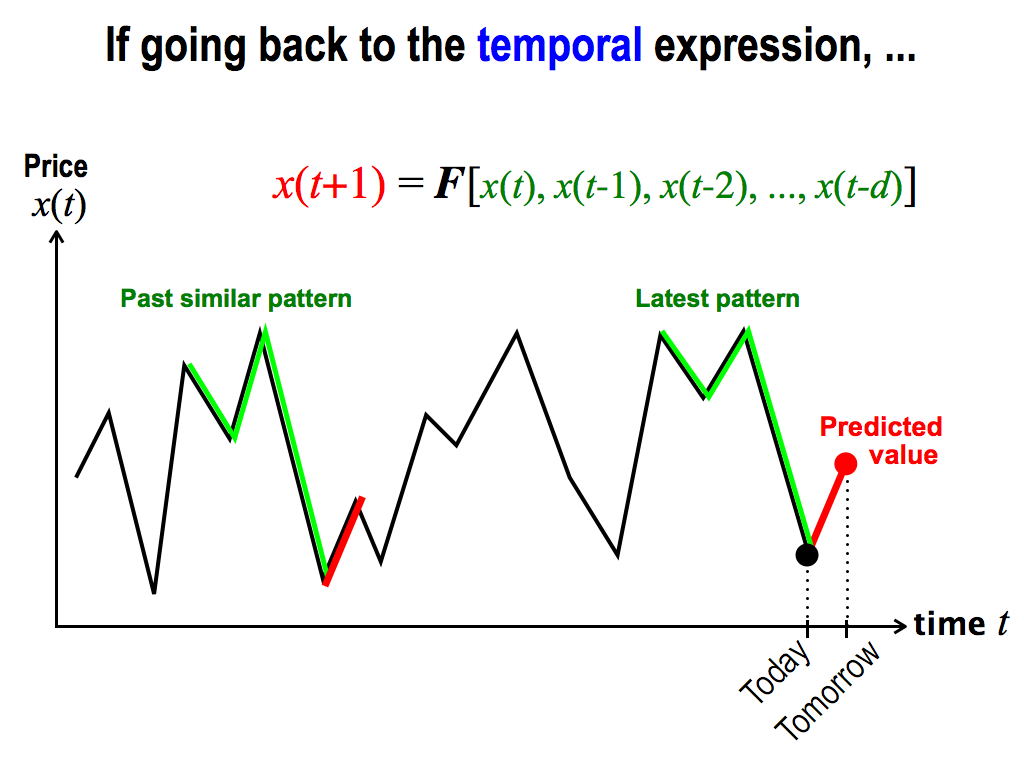
So, what I have to do is, only to follow this movement to calculate this predicted value. This is the same as the chaos prediction.
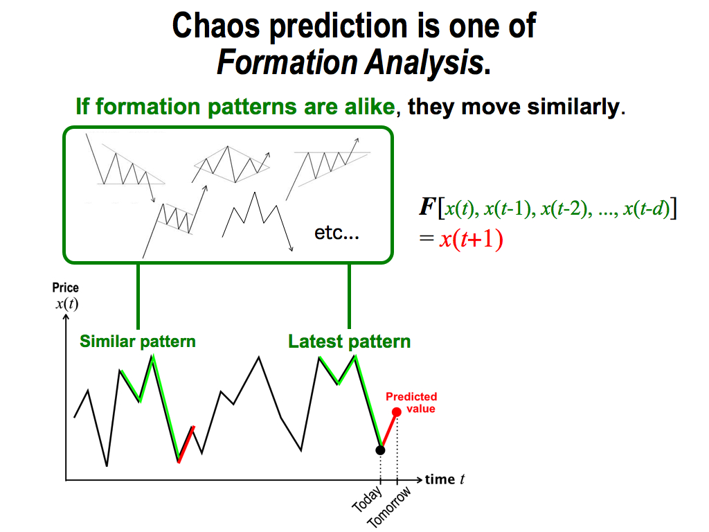
Actually, we can consider that this chaos prediction is one of the formation analysis. As you know, there are famous patterns like these in the formation analysis.
This expression “If formation patterns are alike” means similar inputs to this function F. Therefore, outputs are also similar. This means “they move similarly.” This is very natural from the viewpoint of chaos theory, So, chaos theory is very familiar with technical analysis and one of the formation analysis.
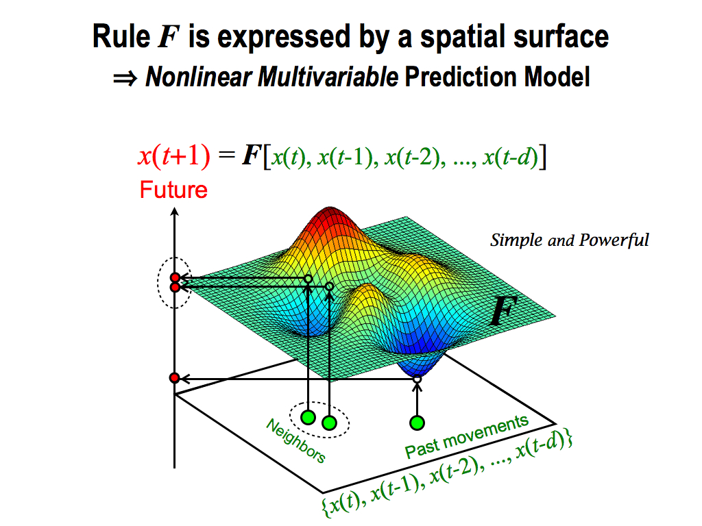
On top of that, this prediction method is very simple and powerful, because this prediction is categorized as a nonlinear multivariable prediction model. This is the highest level of prediction models.
Here, rule F is expressed by a spatial surface. Surface means nonlinear. If it’s linear, we can use only plain to express the rule F. Linear model isn’t powerful. Then, this function F has some inputs. That’s why, it’s multivariable.
Finally, these neighbors are similar inputs to the function F. So, their outputs are also similar, because the rule F is the relationship between past and future. This is the key-point of this prediction model.
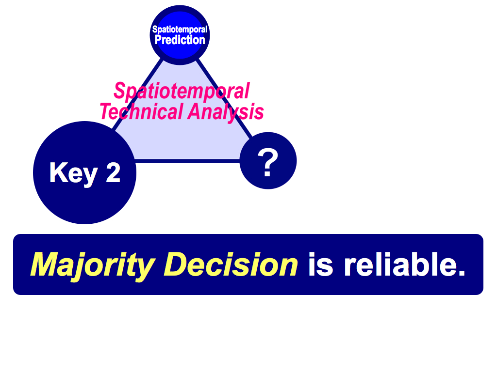
Next key is majority decision, which is so reliable to improve prediction accuracy.
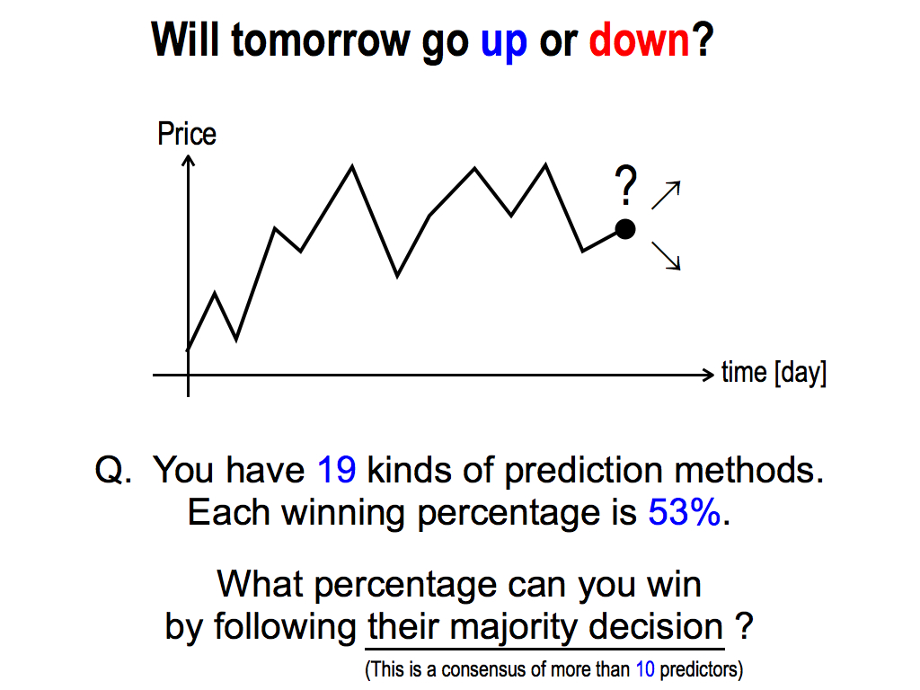
Here, I have another question. Will tomorrow’s price go up or down? This is an alternative question.
To consider this question, please think of this situation, you have 19 kinds of prediction methods. Each winning percentage is 53%. This is a bit more than 50%. 50% is the chance level, because this question is alternative. So, each prediction method can predict future just a little bit.
My question is, What percentage can you win by following their majority decision? This is a consensus of more than 10 predictors, because the total is 19. 10 is more than half. So, this is the majority decision.
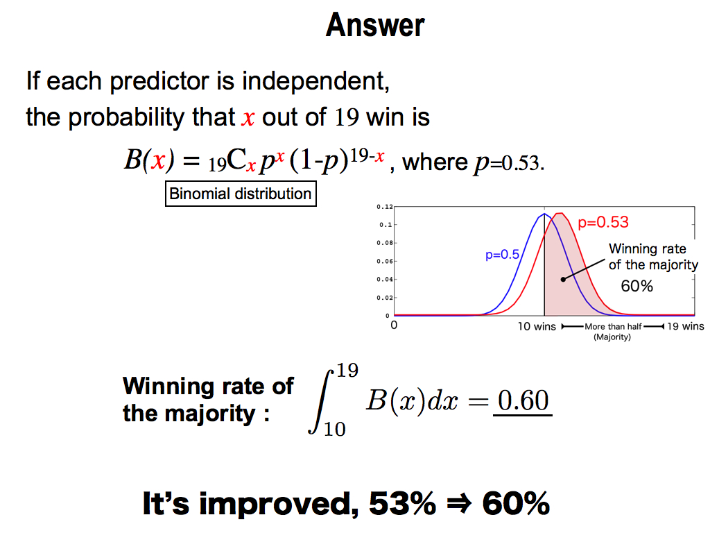
This is the answer. According to Statistics, it each predictor is independent, the probability that x out of 19 predictors win is the binomial distribution. And therefore, winning rate of the majority can be calculated by the integral of more than 10 wins. This is the area of the red region. Its answer is 0.6. It’s amazing that the winning rate is improved to 60% from the initial 53%. This improvement is dramatic. This is the power of majority.
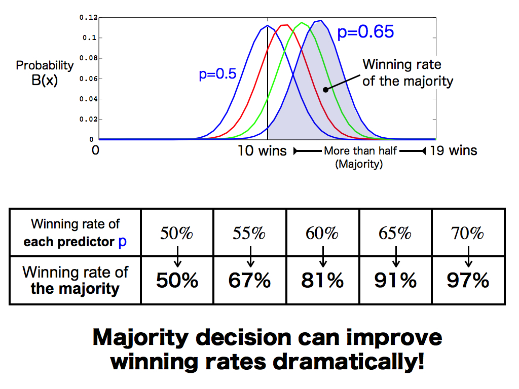
Then, to consider this majority power in more detail, I changed the initial winning rate of each predictor p from 50% to 70%. Of course, if it’s 50%, their majority cannot improve winning rate. But, if this initial winning rate is a bit more than 50%, their majority decision can improve winning rates dramatically, like these. This is the power of the majority decision. And, in the field of data mining, this is called as the ensemble learning.
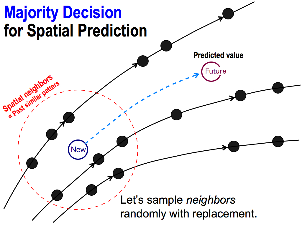
So, I want to apply this majority power for my spatial prediction. For this purpose, we have to reproduce lots of predictors. So, this is my idea: let’s sample these neighbors randomly with replacement…
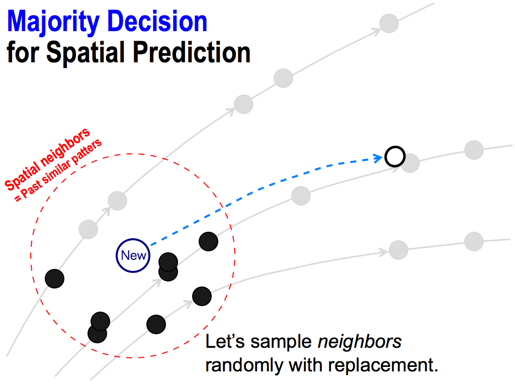
... like this. Each neighbor can be selected many times. In this case, lower neighbors were selected, and therefore the predicted value goes down.
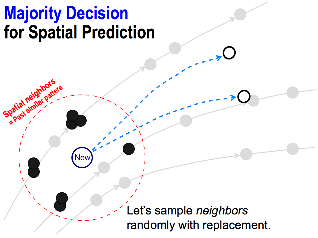
This procedure is repeated many times. In this case, upper neighbors were selected. So, the predicted value goes up.
And next, I got another predicted value.
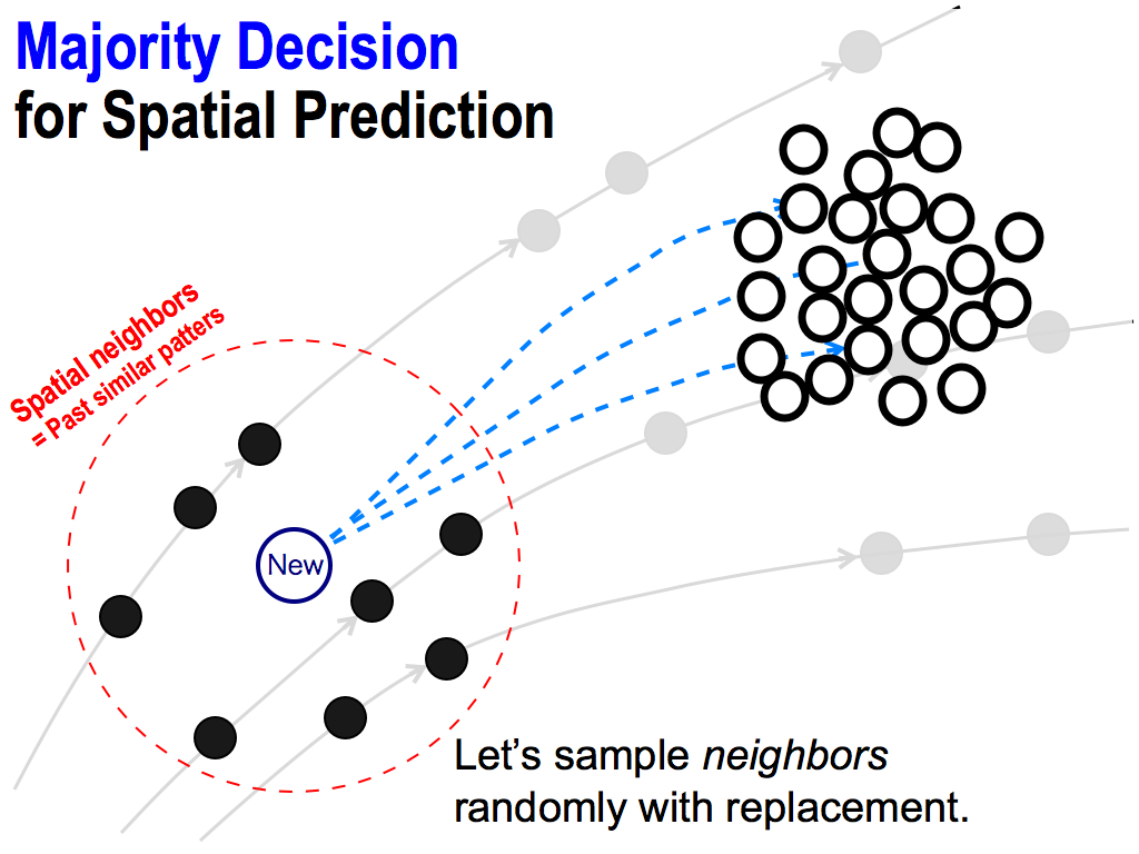
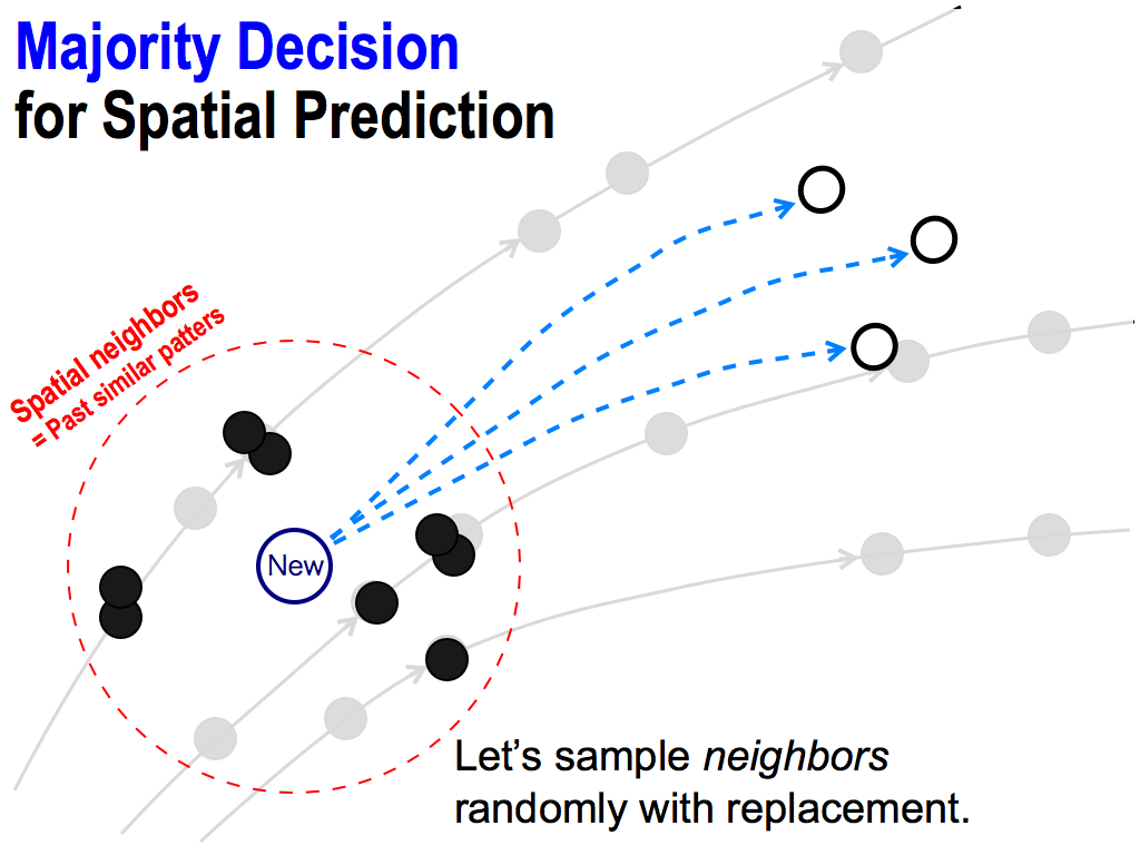
By repeating this, I can get lots of predicted values. These are opinions of each predictor.
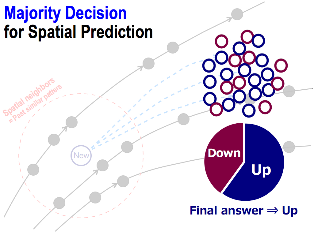
And then, I count these opinions like this. If the number of up’s opinions is more than down’s, let’s consider the final predicted answer is UP. This is a majority decision. This is the consensus of the majority.
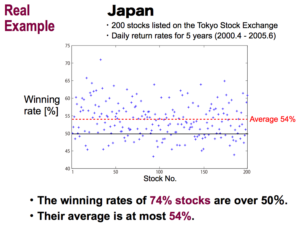
Ok, let me show you a real example of Japan. I used 200 stocks listed on the Tokyo Stock Exchange, and predicted daily return rates for 5 years. Vertical axis means the winning rate. Horizontal axis means stock number.
This prediction is alternative of up or down. So, 50% is the chance level. As results, the winning rates of 74% stocks are over 50%, over the chance level. It’s a good result. But, their average shown here is at most 54%. So, real market is difficult to predict.
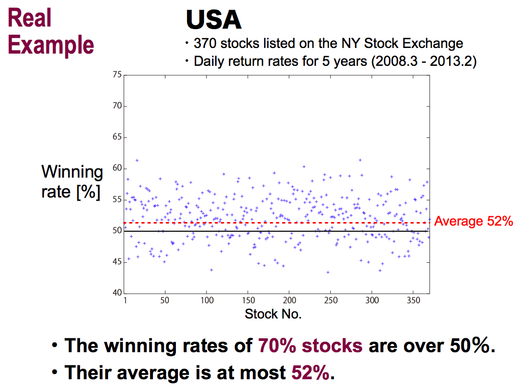
This is the result of the USA, I used 370 stocks listed on the NY stock exchange, and predicted daily return rates for 5 years. As wall as Japan, the winning rates of 70% stocks are over the chance level. This is good, but their average is at most 52%. It’s not high as well as Japan...
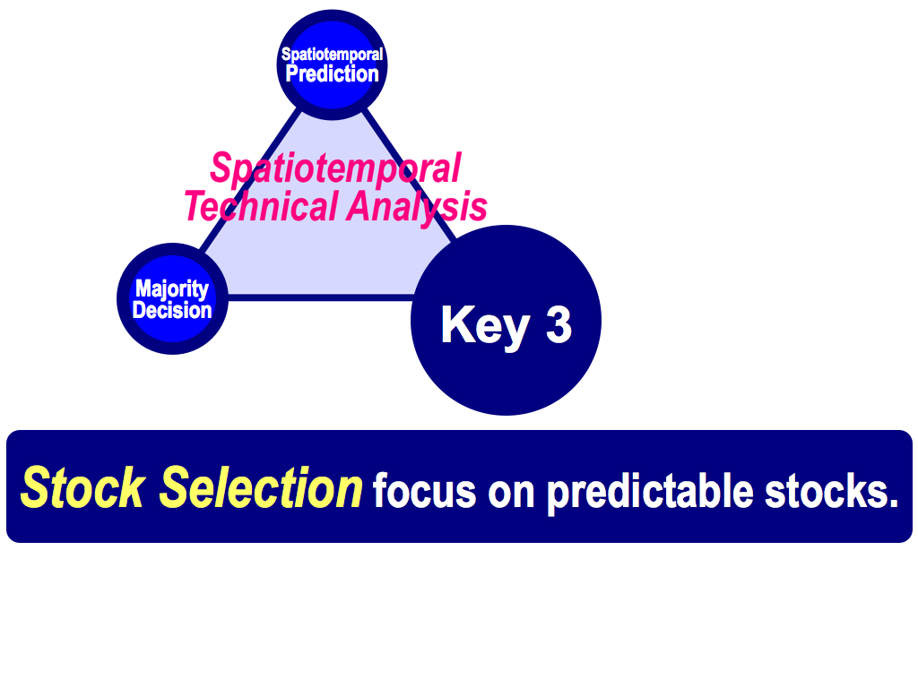
So, in order to improve prediction accuracy, we have to use the third key. This is Stock Selection to focus on predictable stocks.
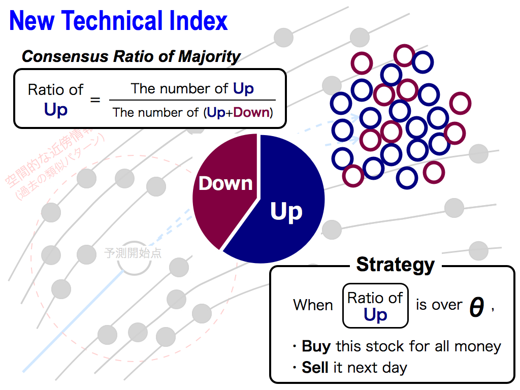
Here, I’d like to propose a new technical index, which is Consensus Ratio of the Majority. This is the ratio of Up’s opinions. So, the number of Ups opinions is divided by the total number of (Ups and Downs) opinions.
And then, investment strategy is very simple. When this ratio is over a threshold θ, namely, we have a high consensus and a high confidence in prediction, I buy this predicted stock for all money, and sell it next day.
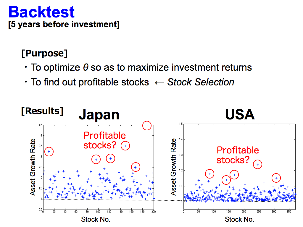
And, backtest is very important in order to optimize θ so as to maximize investment returns, and to find out profitable stocks. This is Stock Selection.
As you can see, this vertical axis means Asset Growth Rate, and the horizontal axis means Stock Number. So, you can see some profitable stocks like these, because their asset growth rates are larger than others. However, this is the backtest. Actually, I don’t know if these stocks are profitable after the backtest.
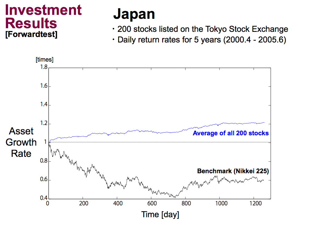
Therefore, I performed Investment simulations as a forwardtest. This is the results of Japan.
Black line means a benchmark of Nikkei average index, and blue line means using my technical index, that is, the consensus ratio of the majority. And, this is the average asset growth rate of all stocks.
As you can see, my technical index is better than benchmark, but still, the asset growth rate is 1.2 times or so.
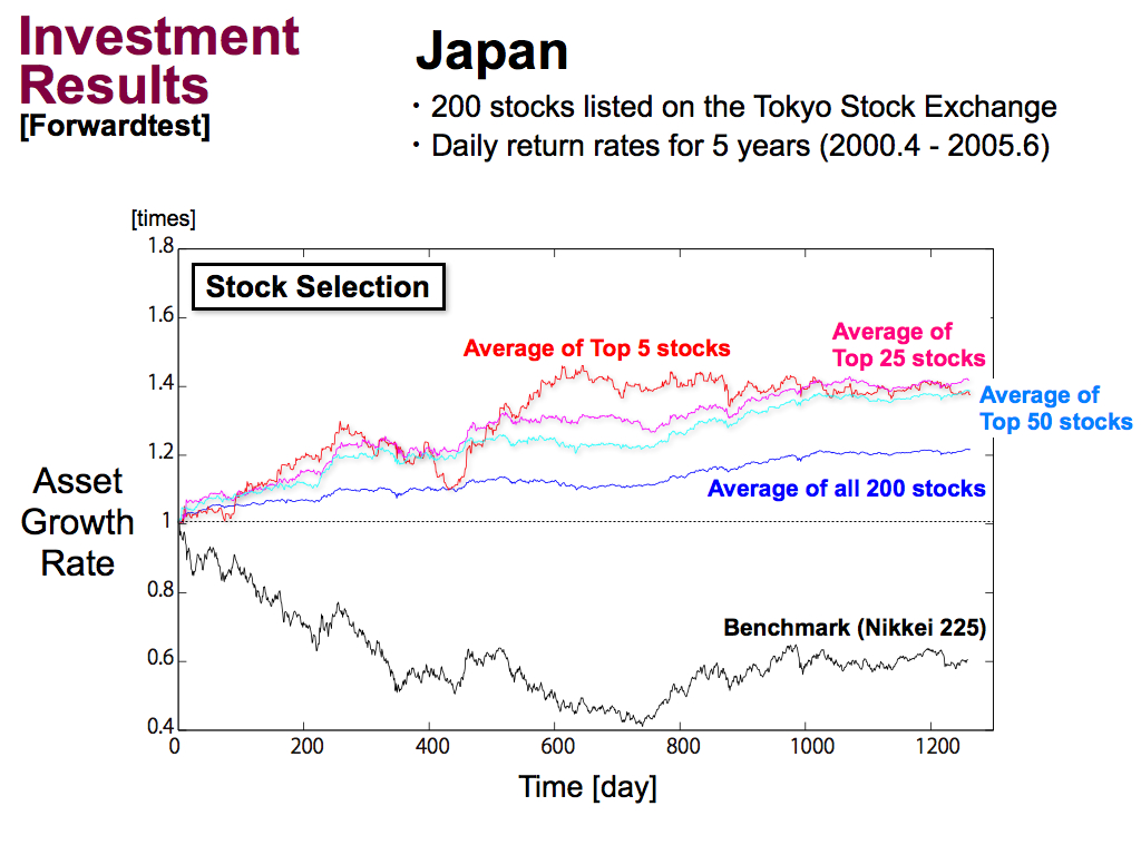
Then, we performed the stock selection, by using Top 5 stocks, using Top 25 stocks, and using Top 50 stocks of the backtest. As you can see, the asset growth rate can be improved by the stock selection.
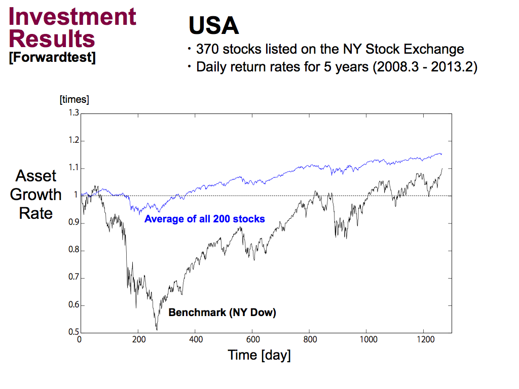
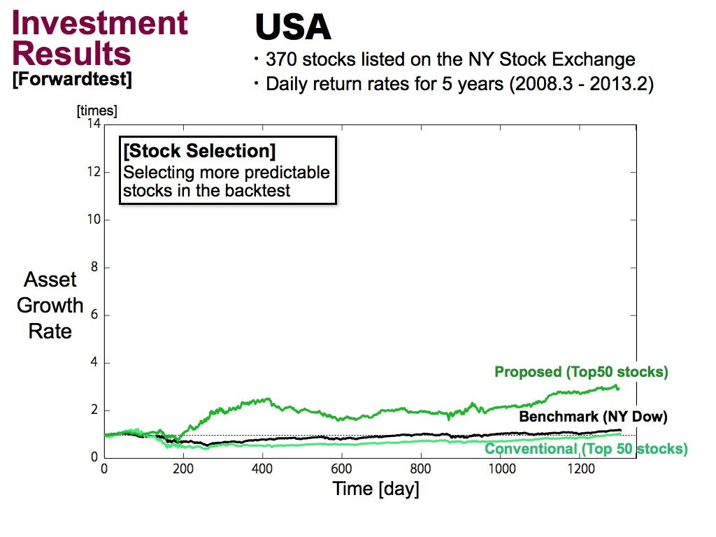
Next is the results of the USA. The benchmark of NY Dow index has a huge draw down. But, my technical index is better than the benchmark.
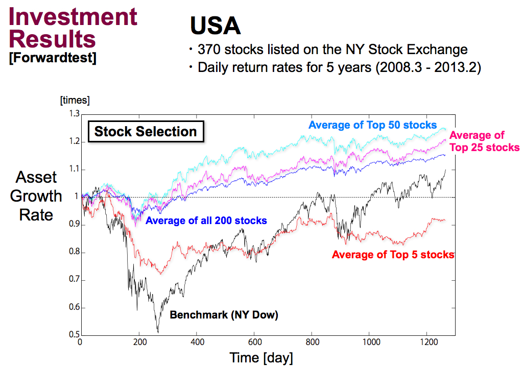
Then, if we applied the stock selection, As well as Japan, stock selection can improve investment performance.
But, using only top 5 stocks is a bit greedy. So, the investment performance was reduced. Namely, it’s better to use some kinds of stocks for stock selection, like Top 50 stocks.
But still, asset growth rate is 1.3 times or so. It’s not high enough. So, to improve investment performance more, ...
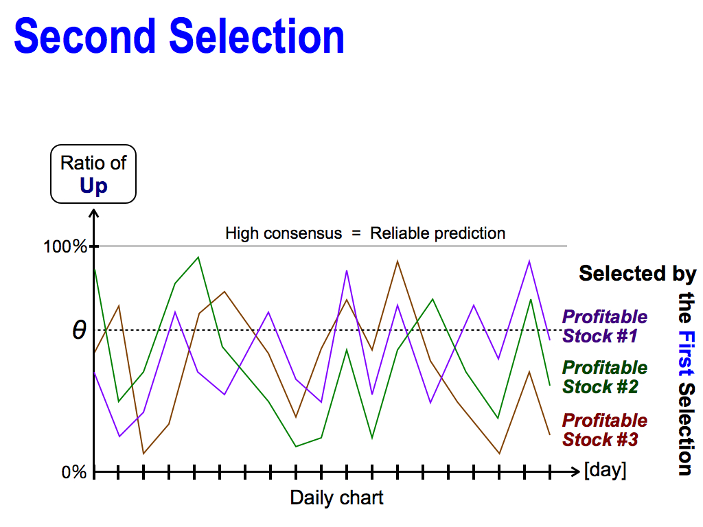
I have one more idea, which is Second Selection. As you can see, these are the profitable stocks selected by the first selection of the backtest. But, each consensus ratio fluctuates everyday. Sometimes, it shows high consensus, which means reliable prediction, but it goes down soon. So, it’s dangerous to believe these stocks.
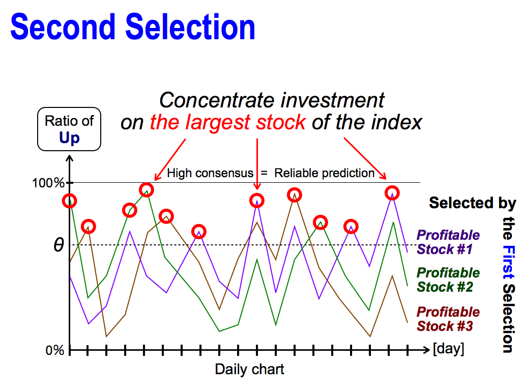
For this reason, it’s better to concentrate investment on the largest stock of the consensus ratio, each day. This is the second selection.
Of course, the first selection is also important as a filter to remove unpredictable stocks before the second selection.
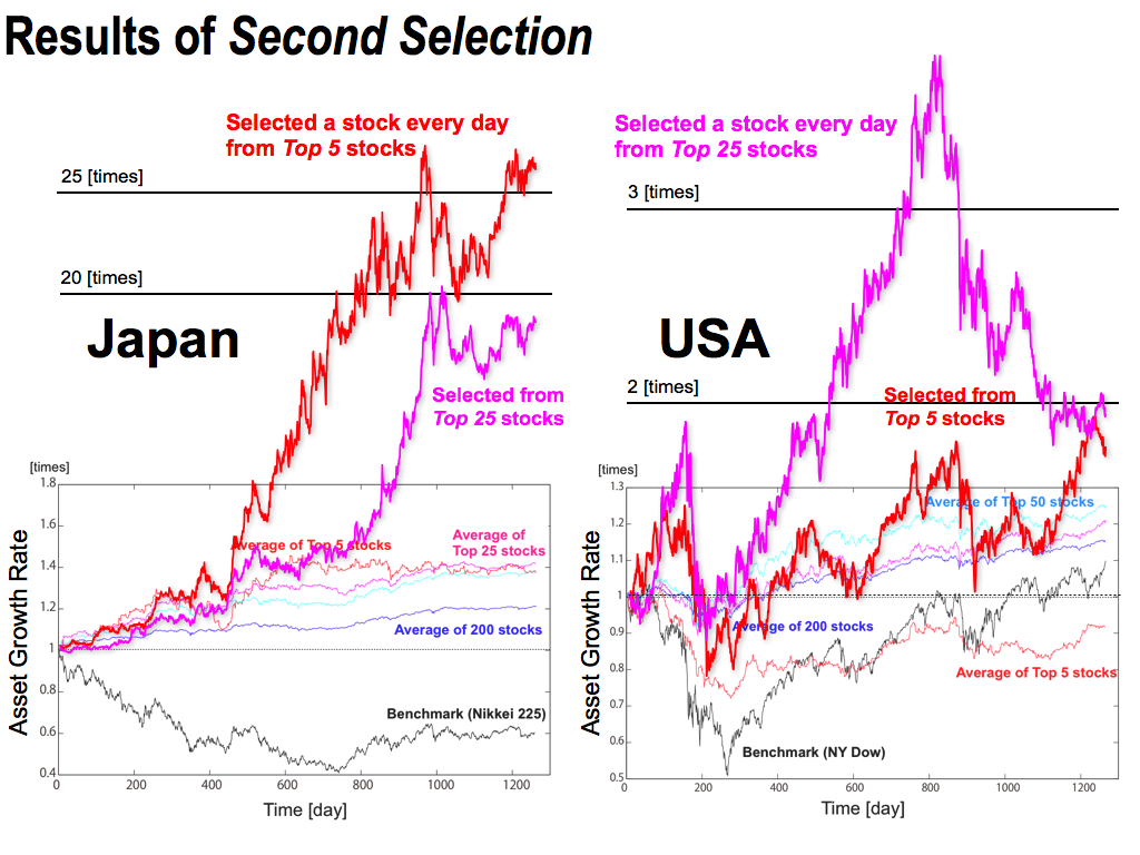
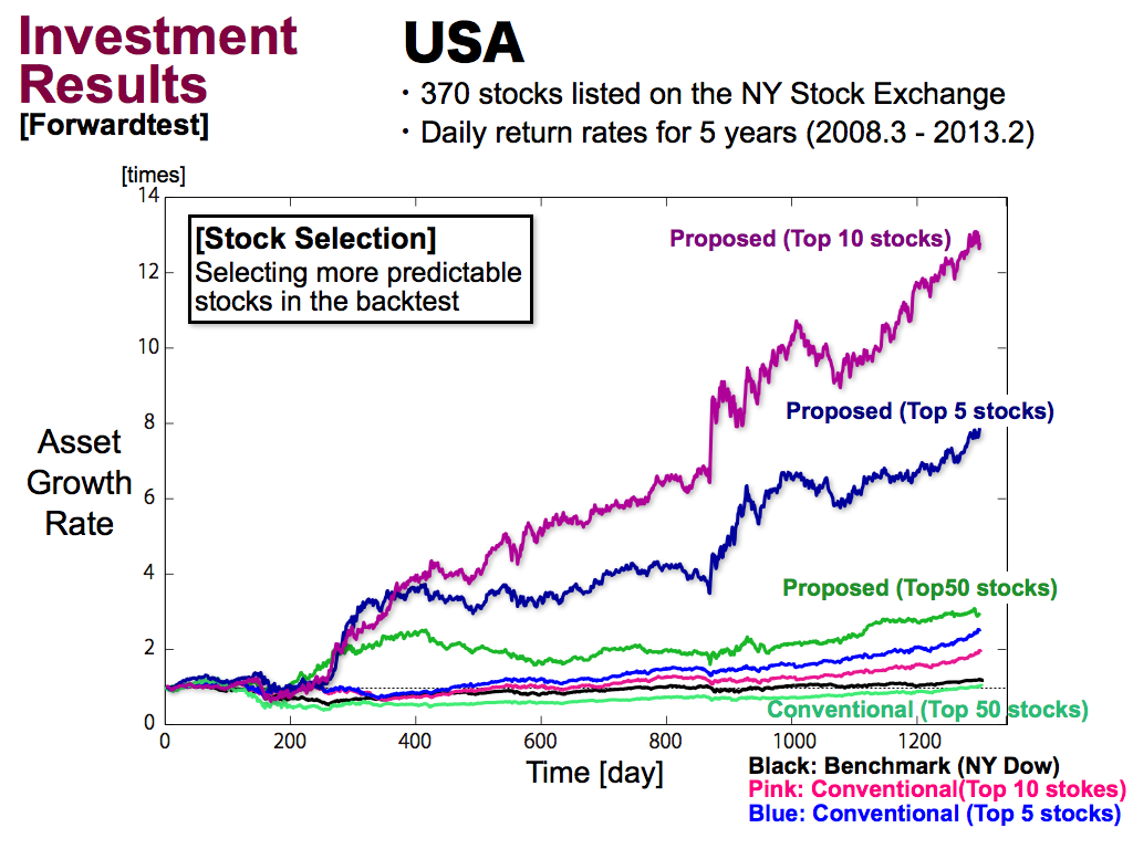
This is the results of the Second Selection. Here, Top 5 stocks or Top 25 stocks were selected by the first selection. After that, I selected the best one stock everyday by the second selection.
As you can see, the second selection can improve the asset growth rate by 25 times in Japan. And, in the USA, there is a huge drawdown, but the asset growth rate is a bit improved by the second selection.
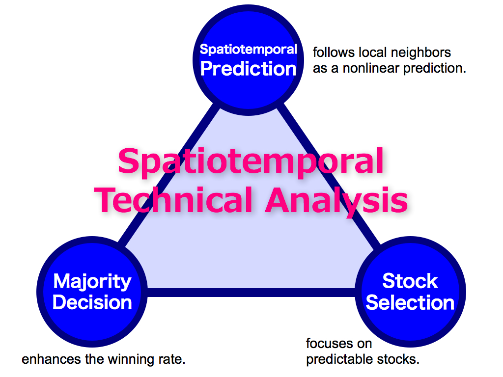
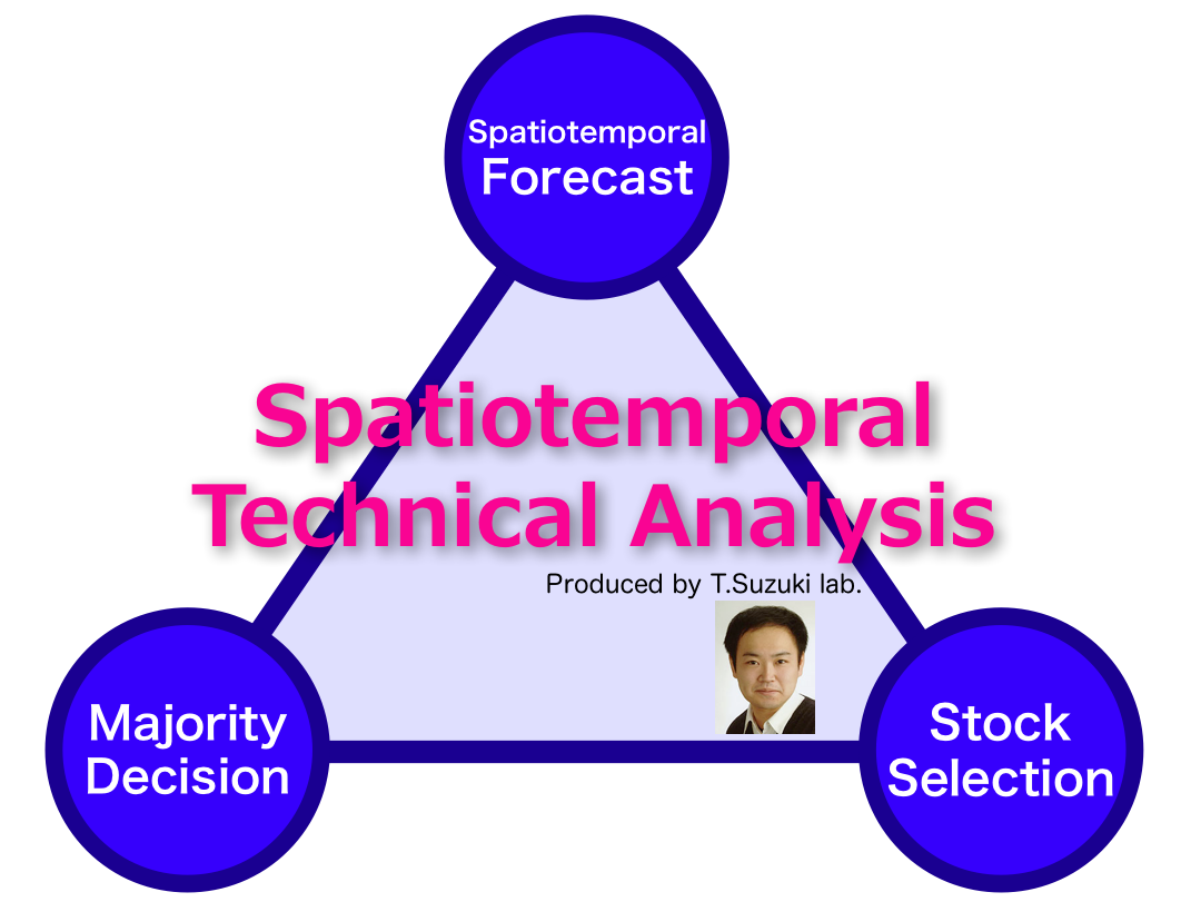
Ok, three key concepts has been completed. The first key is Spatiotemporal Prediction, which follows local neighbors as a nonlinear prediction. This is a simple, but powerful. The second key is Majority Decision, which enhances the winning rate by using the majority power. The third key is Stock Selection, which focuses on predictable stocks by using the first selection and the second selection. This is the framework of my theory. It’s Spatiotemporal Technical Analysis.
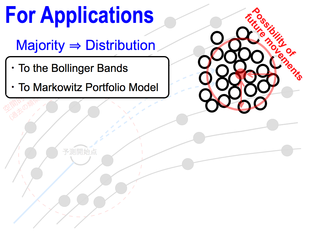
For the next step, I’d like to apply my theory to the Bollinger Bands and Markowitz Portfolio Model.
For these applications, let’s consider this majority opinions as a distribution, which is the possibility of future movements.
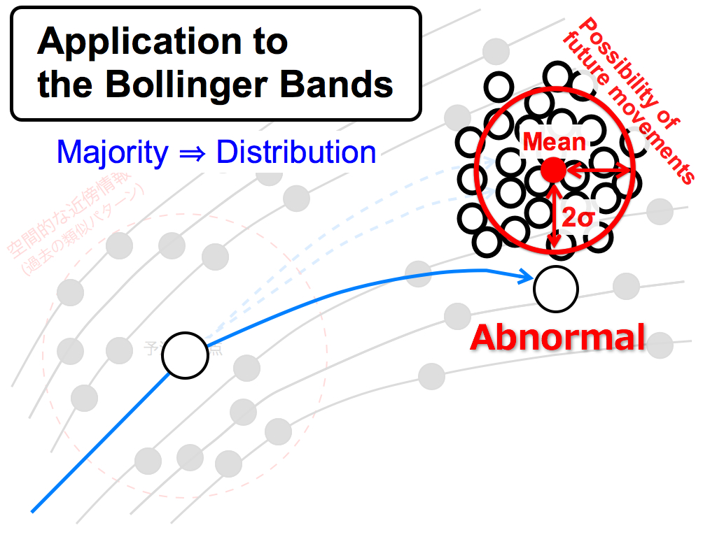
The first application is the Bollinger Bands.
If this spatial movement goes out of 2 sigma of the distribution like this, let’s consider this behavior is abnormal phenomenon in terms of Statistics. This concept is the same as the Bollinger Bands.
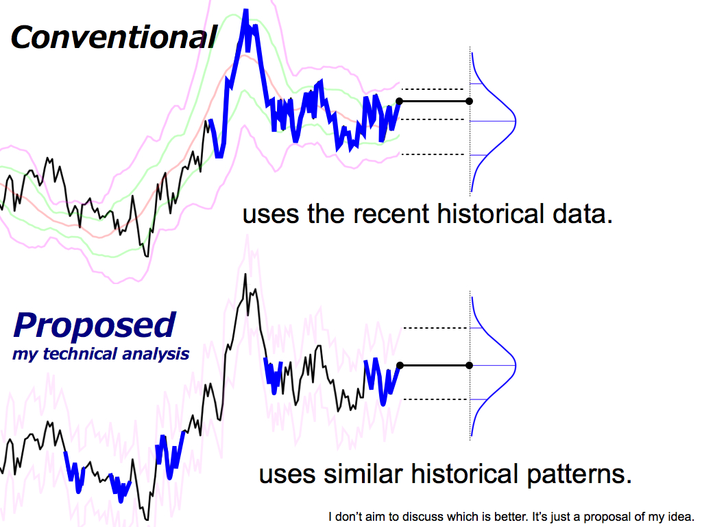
By the way, what is the difference between the conventional method and my proposed method? As you know, the conventional method uses the recent historical data to draw the Bollinger Bands, like this.
On the other hand, my proposed method uses similar historical patterns to predict the future distribution and calculate the Bollinger Bands by using two sigma, like this. But, I don’t want to discuss which is better. It’s just my proposal.
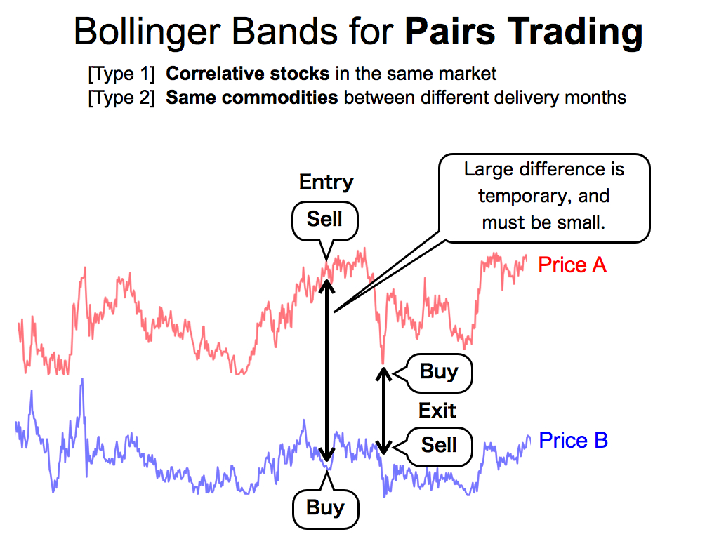
In this study, I use the Bollinger Bands for pairs trading. Pairs trading have some types. The first type is using correlative stocks in the same market. The second type is using the same commodities between different delivery months.
In both types, these two prices of a pair must be synchronized each other because of the law of one price in Economics. Therefore, if there is a large difference like this, it is a temporary phenomenon, and it must be small soon. By using this arbitrage opportunity, we can get profit.
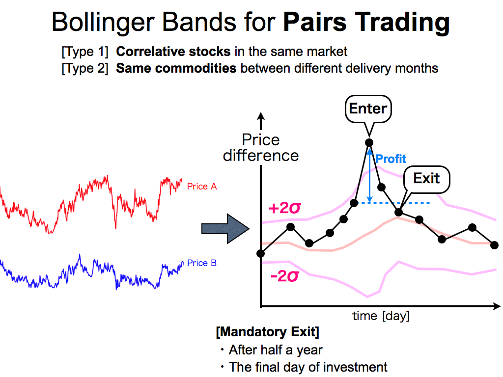
First of all, I make price difference between two prices of a pair like this. Then, if the price difference is over +2 sigma like this, I enter the market. After that, if the price difference is under the value just before this enter, that is, if it becomes under this line, I exit from the market. And, I can get this profit.
Moreover, for risk management, we have to consider mandatory exit rules. if I can’t exit from the market after half a year or by the final day of investment, I close the position, mandatory.

This is investment results of correlative stocks for pairs trading in the USA, I used 1770 pairs on the NY stock exchange of daily prices for 5 years.
Black line means a benchmark of NY Dow index, and blue line means using the conventional Bollinger Bands. Navy blue line means using my proposed Bollinger Bands. These results are the average of all thousand of pairs, and these are better than the benchmark.
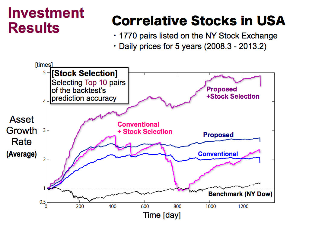
Then, I applied the stock selection by using Top 10 pairs of the backtest’s prediction accuracy. These results are the average of the selected Top 10 pairs.
As you can see, asset growth rate can be improved by the stock selection, especially for the proposed method, by about 5 times for 5 years.
On the other hand, for conventional method, this stock selection didn’t work well.
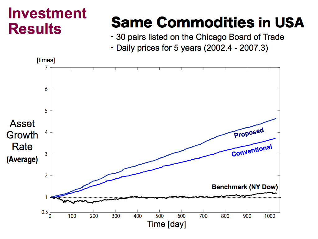
Next is the results of the same commodities in USA. I used 30 pairs of the Chicago market of daily prices for 5 years.
These are the average asset growth rate of all 30 pairs, by the proposed Bollinger bands and the conventional Bollinger Bands. These are better than the benchmark.
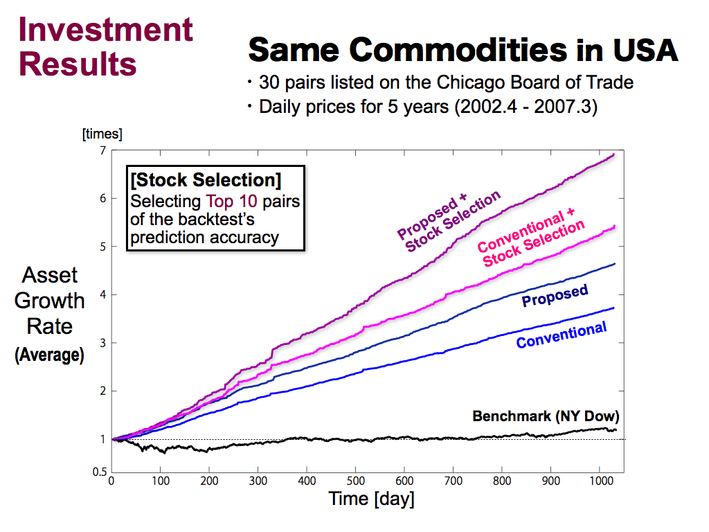
Then, we applied the stock selection. Asset growth rate can be improved by the stock selection by 7 times for 5 years. And, the conventional method was also improved.
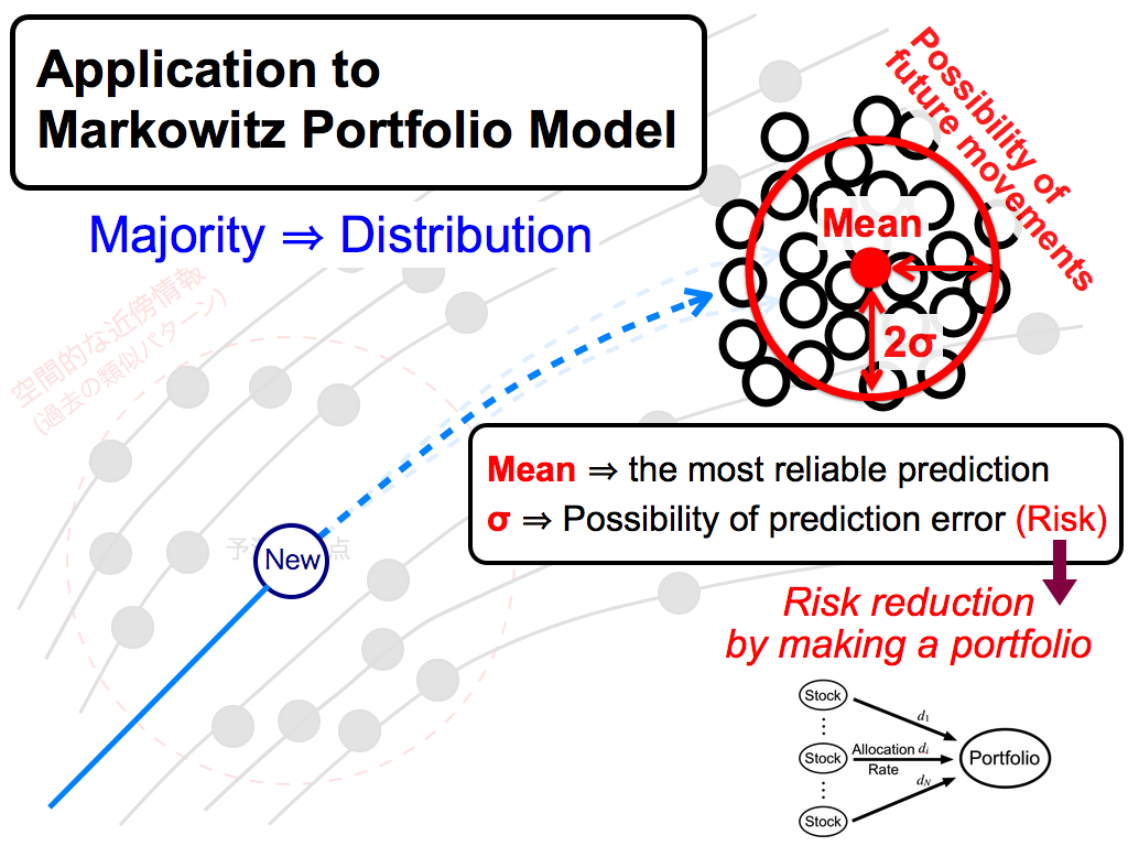
The last application is the portfolio theory.
Here, this distribution can be considered as the possibility of future movements. So, this mean value of the majority corresponds to the most reliable prediction, because it is the consensus of of the majority. And, this standard deviation corresponds to the disagreement of the majority. So, it is the possibility of prediction error. Namely, it's risk. I want to reduce it by making a portfolio.
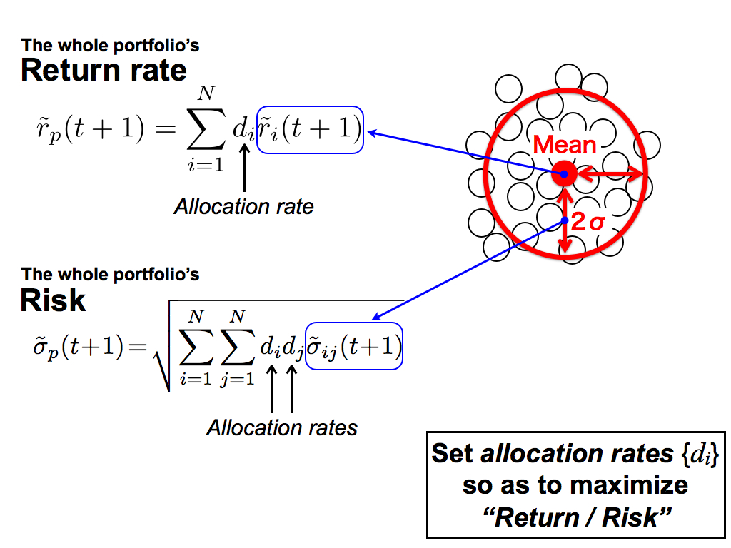
As you know, these equations are part of Markowitz portfolio model. This is the whole portfolio’s return rate. Here, p means the portfolio, and i means the stock index. then, d_i means the allocation rate of i-th stock. This is the whole portfolio’s risk.
To compose a portfolio, we set these allocation rates, so as to maximize this ratio, the return rate divided by the risk.
In my theory, this mean value of the majority is the most reliable predicted value. So, I use it for this expected future return. And, this standard deviation means the disagreement of the majority and the prediction risk. So, I use it for this expected risk.
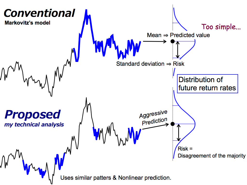
Then, this is the difference between the conventional portfolio model and my proposed model.
As you know, the conventional model uses the recent historical data to make a distribution of future return rates. And, the mean value is the predicted future return, and the standard deviation is the risk. So, this idea is too simple from the viewpoint of prediction. Predicted value is nothing but the moving average.
On the other hand, my proposed method uses historical similar patterns to predict the future return rates aggressively, by using spatial nonlinear prediction like the formation analysis.
Then, this risk means the disagreement of the majority, that is, the possibility of prediction error. So, I reduce this prediction risk by making a portfolio.
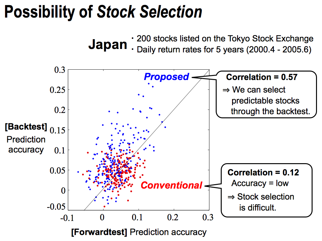
Moreover, before investment simulations, I want to check on the possibility of Stock Selection. The vertical axis is the backtest’s prediction accuracy, and the horizontal axis is the forawardtest’s prediction accuracy. But, we cannot see the result of the forwardtest, before starting actual investments. So, if there is some correlation between them, we can select predictable stocks through the backtest.
As you can see, my proposed method has a good correlation 0.57. This means the Stock Selection is possible to some degree.
However, the conventional method has a slight correlation. And, its prediction accuracy is small as shown here because this prediction method is too simple. So, stock selection might be difficult.
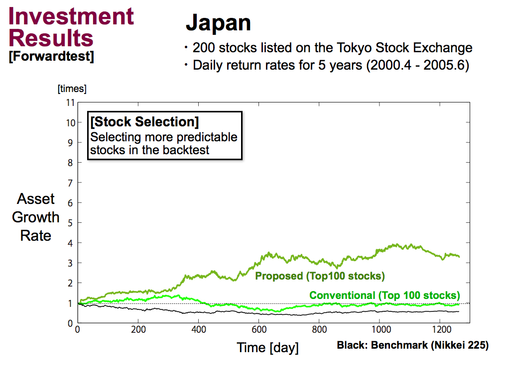
This is the investment results of the forwardtest in Japan. Black line means a benchmark, and green line means the conventional portfolio model using top 100 stocks selected by the backtest. Then, navy green line means my proposed portfolio model. These are better than the benchmark.
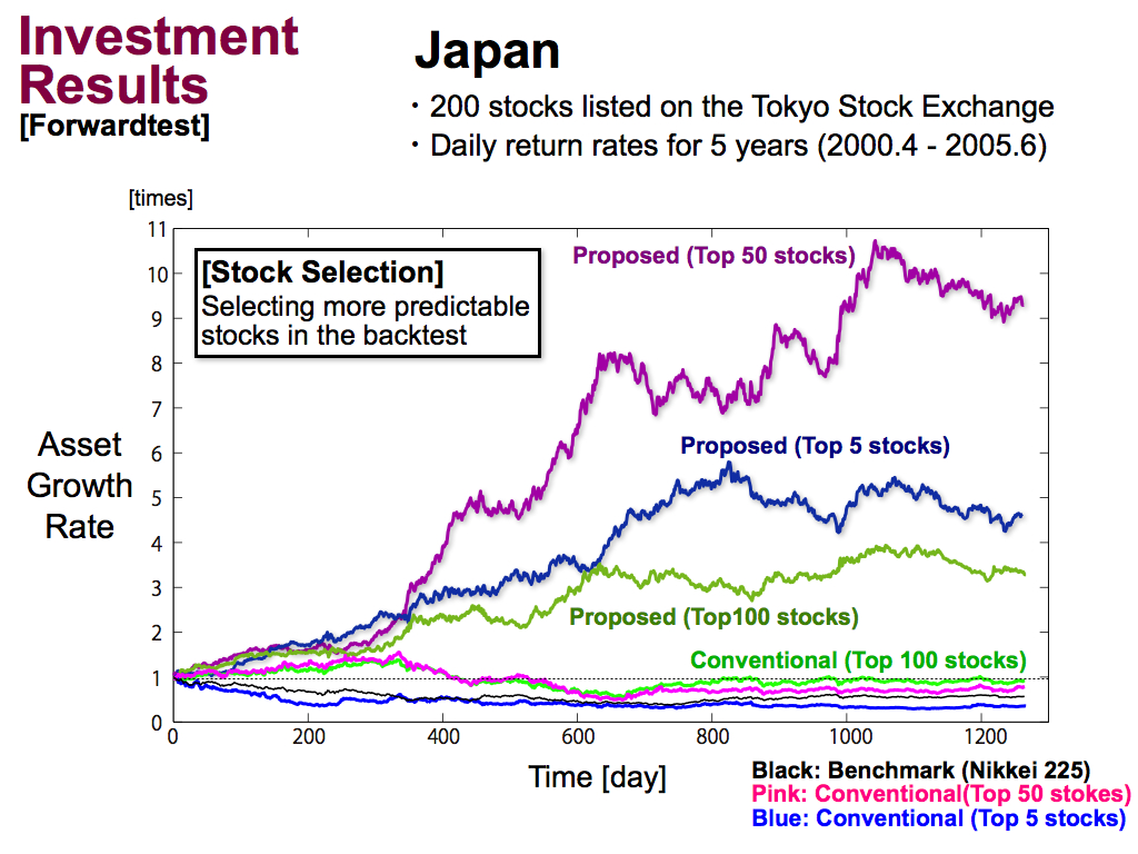
We performed stock selection more greedily, like using only top 50 or only top 5. As a result, the asset growth rate is improved by around 10 times for 5 years, for my proposed portfolio model.
However, using only Top 5 stocks is a bit greedy. So, this performance was reduced. And, it’s better to use some kinds of stocks to make a portfolio, like using Top 50 stocks, like this.
On the other hand, for conventional portfolio model, the stock selection didn’t work at all as I expected in the previous slide.
Then, this is results of the USA. As well as Japan, the proposed method works better.
Then, if we performed stock selection more greedily, we can improve the asset growth rate of my proposed model by around 14 times.
But, for the conventional portfolio model, the stock selection didn’t work at all as well as Japan.
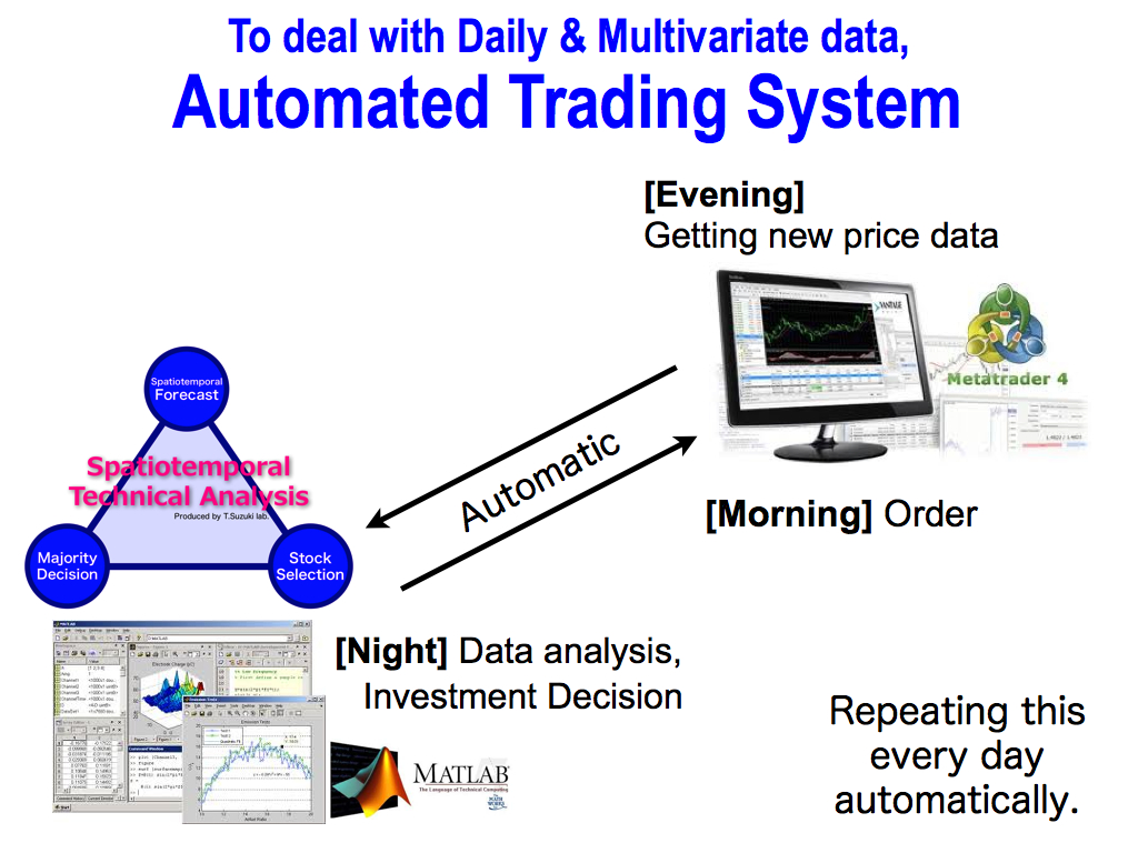
Finally, I’d like to introduce an example of automated trading system, because our method has to deal with daily data and multivariate data everyday. It’s very hard for human to do that.
As you know, Metatrader is a famous free tool to make an automated trading system. But, the way of programing is a bit unique, and it is sometimes changed by releasing a new version. So, I don’t want to use it mainly. I use it only for getting new price data and order.
In stead of that, I use Matlab for data analysis. Matlab is a standard programing software. Then, my laboratory made a system to connect them automatically and repeat this investment process: getting data in the evening, data analysis at night, and order in the next morning, every day automatically.
That’s all. Thank you for your attention. If you have any questions and comments, please send E-mail to me.
Finally, this is the framework of my method again. Thank you.
Q & A
Q. Are real markets are actually chaos?A. As you know, nobody found a strong evidence of chaos. That's why, chaos boom was over in Economics. However, I think that markets are sometimes chaotic, but often stochastic like the random walk. So, what we can do is to grasp the rare profitable chance of chaotic or deterministic markets.
My method of "Consensus ratio of the majority" is based on this concept. So, only when we have high consensus and high confidence in prediction, I enter the market.
Q. Why is the period of the backtest and forwardtest only five years? Isn't it short?
A. I think that the structure of markets is sometimes changed by huge accidents such as earth quake, Lehman crash, and bubble economy, etc. So, I don't want to use long historical data. I want to use the same market structure for data analysis and for prediction.
Q. Why did you use dairy data?
A. According to our previous studies, weekly and monthly data are more difficult to predict than dairy data. I think, weekly and monthly data are stochastic process, while dairy data might have a slight deterministic process like the rule F. So, dairy data is a bit easier to be predicted than longer-term data.
On the other hand, I don't prefer shorter-term data like tick data because trading commission is increased very much, and I need to take care the liquidity risk.
Others
If you have a Facebook account, please be my friend on the Facebook(https://www.facebook.com/suzuki.tomoya)
and share with anything about financial markets and technical analysis!
Newest Paper
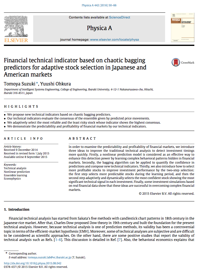 T. Suzuki, Y. Ohkura: Physica A 442, 2016
 H. Koizumi, T.Suzuki: TA Journal 2, 2015
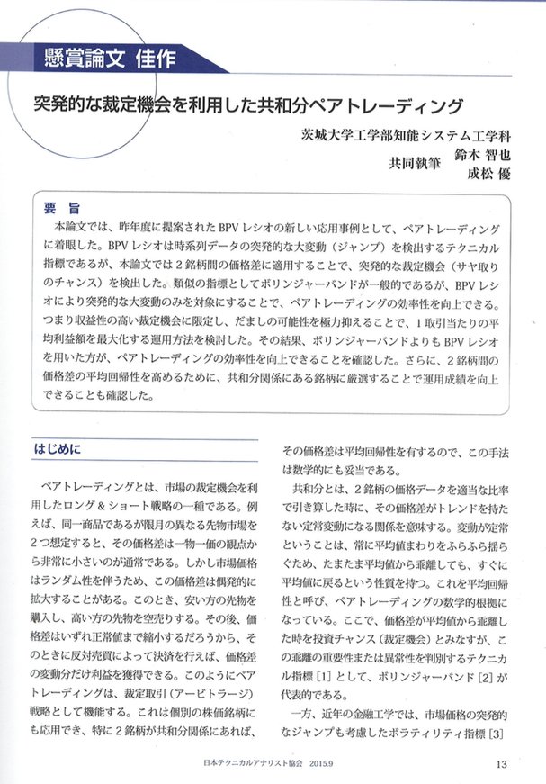 T.Suzuki, M. Narimatsu: TA Journal 2, 2015
Research Image
Detail is shown here.
Predicting future behavior of a complex real system by analyzing its historical time-series data
Recent Paper
 T. Suzuki, K. Ohkura, and M. Okazawa: int. J of Modern Phys. C 26(11), 2015
 T.Suzuki: JSP 16(6), 2012
 Y. Otsuka, T.Suzuki: TOM 5(1), 2012
 T.Suzuki: PRE 83(6), 2011
 Y.Ueoka, T.Suzuki, S.Yamamoto: Int.J.Mod.Phys.C 21(8), 2010
 T.Suzuki, Y.Ueoka, H.Sato: PRE 80(6), 2009